PS Exam Preparation

Comprehensive preparation for the NCEES Principles and Practice of Surveying (PS) exam. 5 modules covering all 5 exam domains with 50 in-depth topics.

Progress0/50

Lesson 3

Data Collection Protocols

Learning Objectives

After completing this topic, you should be able to:

Design data collection protocols appropriate to survey type and accuracy requirements
Implement field-to-finish workflows using feature coding systems
Apply quality control procedures including redundant measurements and closure checks
Distinguish between blunders, systematic errors, and random errors in field data
Evaluate data quality through statistical measures and rejection criteria
Establish procedures for data management, backup, and archiving

Overview

Data collection is the bridge between field measurement and final deliverables. A well-designed data collection protocol ensures that measurements are complete, accurate, properly coded, and ready for efficient processing. Poor data collection practices lead to return trips to the field, processing delays, and errors in the final product.

Modern surveying uses electronic data collectors that store observations digitally and apply real-time computations. However, the electronic format does not eliminate the need for careful planning, systematic procedures, and rigorous quality control. The data collector is a tool; the surveyor's judgment determines how well it is used.

Key Concepts

Figure PS.2.3 — Data Collection and Quality Control Workflow

Data Collection Planning

Before beginning field work, the surveyor should develop a data collection plan that addresses:

Planning Element	Considerations
Project requirements	Accuracy standards, deliverable specifications, scope of work
Measurement methods	Total station, GPS, level, combination
Control framework	Existing control, new control needed, datum and projection
Feature coding	Code list, attribute requirements, line work connections
Quality checks	Closure requirements, redundant observations, check shots
Data management	File naming, backup procedures, transfer protocols
Crew assignments	Party chief responsibilities, instrument operator, rod person

Feature Coding Systems

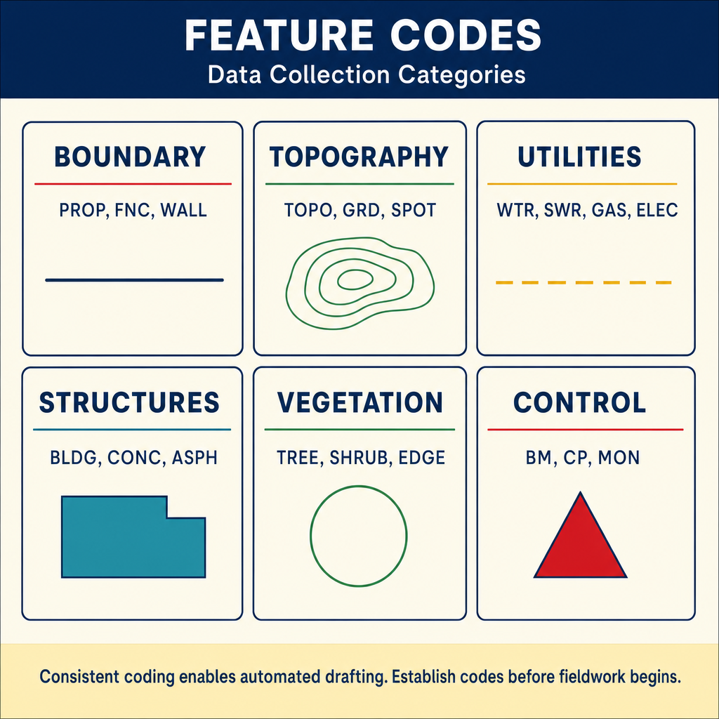
Figure PS.2.21 — Six feature-code categories with examples

Feature coding translates field observations into meaningful geospatial data. A well-designed coding system allows automated processing (field-to-finish) where raw survey points become finished drawings with minimal manual editing.

Code Structure

A typical feature code consists of:

Feature identifier -- a short alphanumeric code representing the feature type (such as EP for edge of pavement, CL for centerline, FL for flow line)
Line control -- codes that start, continue, and end line strings (such as begin, end, curve start, curve end)
Attributes -- additional information such as material, size, condition, or elevation

Example Feature Codes

Code	Feature	Line Behavior
EP	Edge of pavement	Connect sequentially
CL	Centerline	Connect sequentially
FL	Flow line (gutter)	Connect sequentially
TC	Top of curb	Connect sequentially
FNC	Fence	Connect sequentially
BLD	Building corner	Connect to form closed polygon
TREE	Tree	Point feature (no line)
MH	Manhole	Point feature (no line)
PP	Power pole	Point feature (no line)
WV	Water valve	Point feature (no line)
SIGN	Sign	Point feature (no line)
CB	Catch basin	Point feature (no line)

Field-to-Finish Processing

Field-to-finish software uses the feature codes to automatically:

Assign point symbols based on the feature type
Connect points into line work based on line control codes
Place features on appropriate drawing layers
Generate labels and annotation
Create surface models from topographic data

The efficiency of field-to-finish depends entirely on consistent, correct coding in the field. Training crew members on the coding system before starting a project is essential.

Quality Control in the Field

Redundant Measurements

Redundancy is the foundation of quality control. Every critical measurement should be verified through independent observation:

Method	Application
Closing the horizon	Measure all angles around a point; should sum to 360 degrees
Closing the traverse	Compare computed closure to measured closure
Check shots to known points	Re-observe previously established points from new setups
Multiple sets of angles	Observe angles in multiple sets for averaging
Reciprocal observations	Measure from both ends (for leveling or trigonometric heights)
Tie to control	Check survey against established control network

Closure Standards

Closure requirements vary by project type and governing standards:

Survey Type	Typical Linear Closure	Typical Angular Closure
Boundary survey (urban)	1:15,000 or better	10 seconds x square root of n
Boundary survey (rural)	1:10,000 or better	15 seconds x square root of n
ALTA/NSPS survey	1:15,000 or better	Per positional tolerance
Topographic survey	1:5,000 to 1:10,000	30 seconds x square root of n
Construction staking	Varies by specification	Varies by specification
Geodetic control	1:100,000 or better	1-3 seconds x square root of n

Blunder Detection

Blunders are gross errors caused by mistakes -- wrong prism height, wrong point number, reading to the wrong target. Unlike random errors, blunders are not reduced by averaging and must be detected and eliminated.

Common blunder sources and detection methods:

Blunder	Detection
Wrong prism/target height	Check heights at each setup, verify in field notes
Transposed digits in reading	Independent re-measurement
Wrong point sighted	Verify target identification, check shot to known point
Incorrect atmospheric data	Compare conditions to nearby weather stations
Wrong prism constant	Verify against known distance
Incorrect station coordinates	Check inverse to adjacent known stations

Statistical Evaluation

When a data set contains redundant observations, statistical methods help evaluate quality:

Standard deviation measures the spread of repeated observations around the mean. For a series of n observations of the same quantity, the standard deviation of a single observation is calculated from the residuals (differences between individual observations and the mean).

Standard error of the mean is the standard deviation divided by the square root of n, representing the expected accuracy of the mean value.

Rejection criteria help identify observations that may contain blunders. Common approaches include:

Reject observations exceeding 3 times the standard deviation from the mean
Apply the modified Thompson tau criterion for small sample sizes
Use the Chi-square test to evaluate whether residuals are consistent with expected random error

Common wrong path — mechanically applying 3-sigma without context. The "3-sigma rule" is a useful first-cut filter for blunders, but applied blindly it rejects legitimate outliers and accepts blunders hidden in the data. Two cautions: (1) The standard deviation is computed from the observations themselves — if one observation is a gross blunder, it inflates the standard deviation, potentially masking itself by pulling the 3-sigma threshold out beyond its own deviation. Robust estimators (median, MAD) or iterative rejection (remove the largest residual, recompute σ, test again) handle this better than one-pass 3-sigma. (2) Small samples have different statistics — for fewer than ~10 observations, the 3-sigma rule is too permissive; use a tau-test or Chauvenet's criterion instead. Exam questions sometimes describe a small dataset (5–8 points) and ask which rejection method is appropriate; the answer is usually a small-sample criterion (tau, Chauvenet's), not 3-sigma.

Quick retrieval check — try before reading on.

▶Eight repeated angle observations yield a standard deviation of 8″. One observation is 22″ from the mean. Under the 3-sigma rule, is this observation rejected? What would a tau-test tell you?

Under 3-sigma: threshold = 3 × 8″ = 24″. The 22″ deviation is just under the threshold, so 3-sigma would not reject it.

Under a small-sample tau-test: for n=8 at a 95% significance level, the critical tau value is approximately 2.39 (from a tau-test table). Threshold = 2.39 × 8″ = 19.1″. The 22″ deviation exceeds 19.1″, so the tau-test would reject the observation.

This illustrates why small-sample criteria matter: 3-sigma is designed for large samples where the standard deviation is well-estimated, but for n=8 the true standard deviation is poorly known and a more conservative threshold is appropriate. Apply 3-sigma for large samples (say n > 30); for smaller samples, use tau, Chauvenet's, or another small-sample criterion. Even better, re-observe the outlier to confirm whether it is a blunder or just bad luck.

Data Management

File Organization

Establish consistent file naming conventions before starting a project:

Include project identifier, date, and instrument/operator identification
Use a sequential numbering system for data files
Maintain a log of all data files created, including content descriptions

Backup Procedures

Data loss can be catastrophic. Implement multiple backup strategies:

Backup Method	Timing	Location
Data collector internal memory	Automatic during collection	On instrument
Download to field computer	Daily, end of field day	Field vehicle or office
Upload to server/cloud	Daily, when connectivity available	Office server or cloud storage
Archive of raw data	At project completion	Long-term storage

Critical rule: Never delete raw data from the data collector until it has been verified on at least one backup medium.

Data Transfer and Processing

The workflow from field to finished product typically follows this sequence:

Download raw data from data collector
Review raw data for completeness and obvious errors
Process traverse computations and adjustments
Apply coordinate transformations if needed
Run field-to-finish to generate line work and symbols
Review the processed data against field notes and sketches
Edit to correct coding errors and add features not auto-generated
Final QC including comparison to control and accuracy assessment

Accuracy vs. Precision

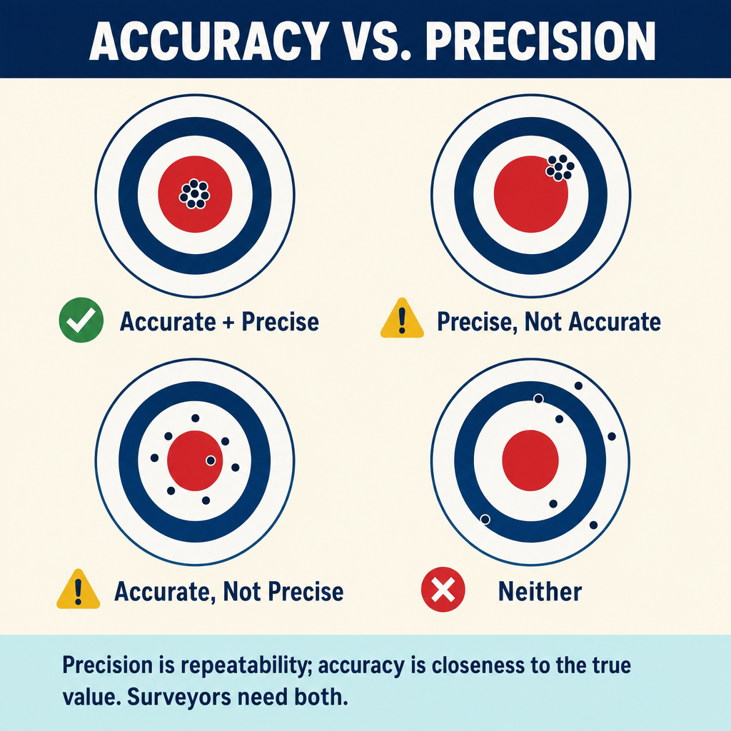
Figure PS.2.20 — Accuracy vs precision (four-target diagram)

Understanding the distinction between accuracy and precision is fundamental to data quality:

Precision refers to the repeatability of measurements -- how closely repeated observations agree with each other. High precision means small random errors.

Accuracy refers to how closely measurements agree with the true value. High accuracy requires both high precision and the absence of systematic errors.

A survey can be precise but inaccurate (if systematic errors are present), or accurate but imprecise (if random errors are large but happen to average out). Professional surveying demands both.

Error Propagation

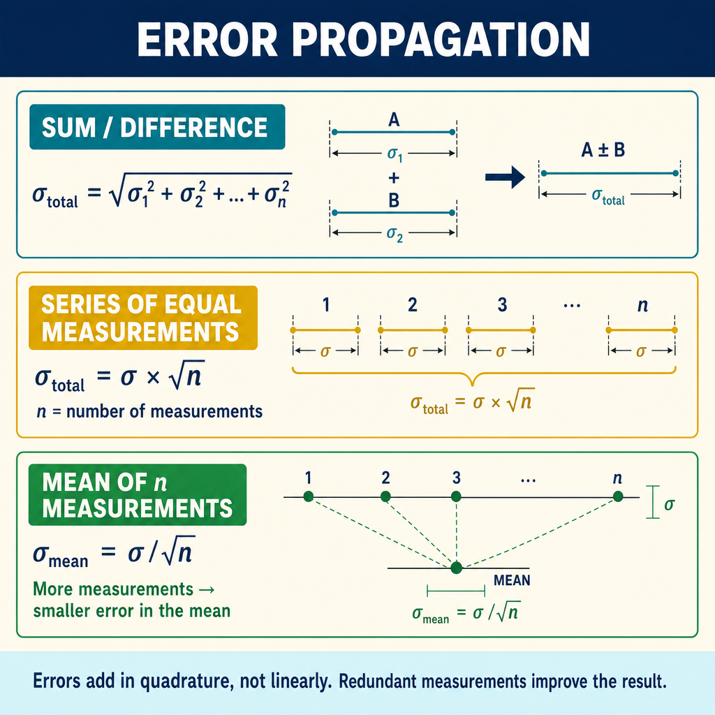
Figure PS.2.22 — Error propagation formulas (sum, series, mean)

When survey measurements are combined through computations (such as computing coordinates from traverse observations), errors in the individual measurements propagate into errors in the computed quantities. Understanding error propagation helps the surveyor:

Predict the expected accuracy of computed results
Design measurement procedures that meet accuracy requirements
Identify which measurements contribute most to overall uncertainty
Allocate measurement effort where it matters most

The general law of propagation of variances states that the variance of a computed quantity is a function of the variances of the input measurements and the partial derivatives of the computation with respect to each input.

Exam Tips

Know the difference between accuracy and precision, and how each is achieved
Redundancy is the key to quality control -- every critical measurement needs an independent check
Blunders are not reduced by averaging and must be detected and removed before adjustment
The 3-sigma rule is a common rejection criterion for identifying potential blunders
Balanced backsight/foresight distances reduce systematic errors in leveling
Field-to-finish efficiency depends on consistent feature coding
Raw field data should never be deleted until verified on backup media
Error propagation determines how individual measurement errors affect final results