PS Exam Preparation

Comprehensive preparation for the NCEES Principles and Practice of Surveying (PS) exam. 5 modules covering all 5 exam domains with 50 in-depth topics.

Progress0/50

Lesson 7

Topographic & Planimetric Mapping

Learning Objectives

After completing this topic, you should be able to:

Distinguish between topographic and planimetric maps
Explain contour line properties, contour intervals, and terrain representation
Describe Digital Terrain Models (DTM) and Triangulated Irregular Networks (TIN)
Identify control requirements for topographic surveys
Explain data collection methods for topographic mapping
Describe data adjustment and quality assurance procedures
Understand mapping scale, resolution, and accuracy relationships

Overview

Topographic mapping represents the three-dimensional surface of the Earth on a two-dimensional medium. A topographic map shows both the horizontal positions of features (planimetric data) and the vertical shape of the terrain through contour lines, spot elevations, and terrain models. These maps serve as the foundation for engineering design, land development, environmental analysis, and construction planning.

The PS exam tests your understanding of contour properties, terrain representation methods, data collection techniques, accuracy standards, and the relationship between map scale and required survey precision.

Key Concepts

Figure PS.5.7 — Contour Line Properties

Topographic vs. Planimetric Maps

Planimetric map:

Shows the horizontal positions of features only
No terrain representation (no contours or elevations)
Features include roads, buildings, boundaries, water bodies, vegetation
Accuracy is assessed in the horizontal plane only

Topographic map:

Shows both horizontal positions and vertical terrain
Includes contour lines, spot elevations, and terrain features
Combines planimetric features with relief representation
Accuracy is assessed in both horizontal and vertical dimensions

Contour Lines

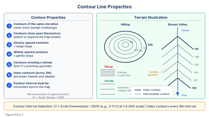
Contour lines are the primary method of representing terrain on a map. Each contour line connects points of equal elevation.

Properties of contour lines:

Contour lines never cross each other (except at overhanging cliffs, which are rare)
Contour lines always close on themselves (though the closure may be beyond the map edge)
Equally spaced contours indicate uniform slope
Closely spaced contours indicate steep terrain
Widely spaced contours indicate gentle terrain
Contour lines form V-shapes pointing upstream when crossing valleys
Contour lines form V-shapes pointing uphill (toward the ridge crest) when crossing ridges
Contour lines are perpendicular to the direction of steepest slope
A closed contour with hachures indicates a depression

Contour interval:

The vertical distance between adjacent contour lines
Selected based on terrain relief, map scale, and intended use
Common intervals: 1, 2, 5, 10, 20, 40, 50, 100 feet (or metric equivalents)
Index contours (every 5th contour) are drawn heavier and labeled with elevation
Supplementary contours (at half the standard interval) may be used in flat areas

Selecting contour interval:

Terrain	Typical Contour Interval
Flat (0-2% slope)	0.5, 1, or 2 feet
Rolling (2-10% slope)	2 or 5 feet
Hilly (10-25% slope)	5 or 10 feet
Mountainous (>25% slope)	10, 20, or 50 feet

Slope from Contour Maps

Slope can be calculated from a contour map:

Slope (%) = (Contour Interval x Number of Contours Crossed) / Map Distance x 100

Or more directly:

Slope (%) = (Elevation Difference / Horizontal Distance) x 100

The direction of steepest slope at any point is perpendicular to the contour line passing through that point.

Digital Terrain Models (DTM) and TIN

Digital Terrain Model (DTM):

A mathematical representation of the terrain surface
Can be grid-based (regularly spaced elevation points) or point-based
Used for volume calculations, cut/fill analysis, drainage design, and visualization
Also called Digital Elevation Model (DEM) when representing bare-earth surface

Triangulated Irregular Network (TIN):

A surface model composed of non-overlapping triangles connecting irregularly spaced points
Each triangle face represents a planar surface with constant slope
Preserves breaklines (ridges, valleys, edges) better than regular grids
More efficient than grids because it uses more points in complex areas and fewer in simple areas
The most common method for engineering-grade terrain modeling

Breaklines:

Linear features that represent abrupt changes in terrain slope
Include ridge lines, valley bottoms, road edges, tops and bottoms of embankments, retaining walls
Must be incorporated into TIN models to accurately represent terrain shape
A TIN without breaklines may produce incorrect interpolation across features

Common wrong path — building a TIN without breaklines. A triangulated irregular network built from elevation points alone (no breaklines) will draw triangles that cross ridges, valleys, and edge features — interpolating the terrain through those abrupt breaks as if they were smooth surfaces. The result: contour lines that cross a ridge as if the ridge weren't there, a stream that appears to run uphill because the TIN averaged across the valley, or a retaining wall whose top-of-wall and toe elevations get smeared into an intermediate slope. Breaklines fix this by forcing triangle edges to follow the linear feature. On the exam, a question that describes poor contour representation at a ridge or abrupt slope change points to missing breaklines — not measurement density, not coordinate accuracy. The solution is to add breaklines where they physically exist, then re-triangulate.

Quick retrieval check — try before reading on.

▶A topographic survey of a small park produces clean elevation points at 50-ft spacing. When you generate contours from the TIN, the contours run in straight lines across a 10-ft-deep drainage ditch as if the ditch weren't there. What's wrong, and how do you fix it?

The TIN was built from elevation points alone, with no breakline for the drainage ditch. When the triangulation algorithm connected points on one side of the ditch to points on the other, it drew triangles whose edges cross the ditch — effectively interpolating the terrain through the ditch at the average of the two top elevations. To fix: add a breakline along the ditch bottom (two linear features: one along each top edge of the ditch plus one along the ditch bottom, or a 3D polyline capturing the channel thread). Retriangulate with the breaklines enforced, and the contours will correctly "dip" into the ditch and back out. No additional field points are needed — the existing points are fine; the problem was the TIN's triangulation rules. This is why boundary surveys for engineering design almost always collect breaklines along ditches, edges of pavement, tops and toes of slopes, and retaining wall faces.

Data Collection Methods

Ground survey (total station or GNSS):

Direct measurement of individual points
Highest accuracy and most control over point selection
Breaklines and critical features are captured explicitly
Most efficient for small to medium-sized sites
Point density determined by terrain complexity and required contour interval

Rule of thumb for point density:

Points should be collected at a density sufficient to accurately define the terrain
Minimum: one point per area equivalent to the contour interval squared (approximately)
Additional points at all breaks in grade, high/low points, and along linear features

Aerial photogrammetry:

Stereo photography processed to extract 3D terrain data
Efficient for large areas
Limited by vegetation cover (cannot see through tree canopy without LiDAR)
Requires ground control points for accuracy
Produces both planimetric features and terrain data

LiDAR (Light Detection and Ranging):

Airborne or terrestrial laser scanning
Extremely high point density (hundreds of points per square meter)
Can penetrate vegetation canopy to reach ground surface
Requires classification of points (ground vs. vegetation vs. structures)
Covered in more detail in Topic 5.8

Control Requirements for Topographic Surveys

Horizontal control:

Primary control established from geodetic network or project control
Control density depends on project size and required accuracy
All topographic data must be tied to the project coordinate system
Minimum of two control points for any survey area (for checking)

Vertical control:

Benchmarks established from geodetic vertical control
Vertical datum must be clearly identified (NAVD 88 preferred)
Closing tolerances depend on the required contour accuracy
Rule of thumb: vertical control must be at least 3 times more accurate than the contour interval

Data Adjustment and Quality Assurance

Field procedures:

Close traverses and level loops before leaving the site
Check random points against control to verify accuracy
Re-measure points that show unusual patterns or potential errors
Document control used, equipment, and calibration dates

Office procedures:

Adjust control networks using least squares or appropriate methods
Review surface models for artifacts and anomalies
Compare spot check elevations against the model
Verify contour representation by comparing with field notes and photographs
Check for correct feature coding and attribution

Quality checks:

Compare independently surveyed check points against the surface model
Verify that contour interval accuracy meets specifications (NMAS or NSSDA)
Check planimetric feature positions against independent measurements
Review edge matching where adjacent survey areas meet

Scale, Resolution, and Accuracy

The relationship between map scale and accuracy is fundamental:

Map Scale	Ground Distance per Inch	Typical Contour Interval	Typical Horizontal Accuracy
1 inch = 10 feet	10 ft	0.5-1 ft	0.33 ft
1 inch = 20 feet	20 ft	1 ft	0.67 ft
1 inch = 50 feet	50 ft	2 ft	1.67 ft
1 inch = 100 feet	100 ft	2-5 ft	3.33 ft
1 inch = 200 feet	200 ft	5 ft	6.67 ft

The horizontal accuracy values above assume NMAS compliance (1/30 inch at map scale for large-scale maps). See Topic 5.13 for detailed NMAS requirements.

Exam Tips

Contour lines never cross (the one exception: overhanging cliffs, which are extremely rare and unlikely to appear on the exam)
Contour V-shapes point upstream in valleys and downhill on ridges
TIN models preserve breaklines better than grid-based models -- this is a key advantage
The vertical accuracy standard under NMAS is: 90% of points tested must be within one-half the contour interval
Slope equals elevation difference divided by horizontal distance, expressed as a percentage
Breaklines are critical for accurate terrain modeling -- without them, TINs produce incorrect interpolation across ridges, valleys, and constructed features
For aerial mapping, ground control points are required to achieve specified accuracy
The relationship between map scale, contour interval, and accuracy requirements is frequently tested
Digital terrain models form the basis for cut/fill analysis, drainage design, and volume calculations in engineering projects

PS Exam Preparation

Module 1: Legal Principles

Module 2: Professional Survey Practices

Module 3: Standards & Specifications

Module 4: Business Practices

Module 5: Areas of Practice