PS Exam Preparation

Comprehensive preparation for the NCEES Principles and Practice of Surveying (PS) exam. 5 modules covering all 5 exam domains with 50 in-depth topics.

Progress0/50

Lesson 5

Surveying Computations

Learning Objectives

After completing this topic, you should be able to:

Perform coordinate geometry (COGO) computations including inversing, intersections, and curve solutions
Apply traverse adjustment methods including compass rule, transit rule, and least squares
Compute areas using coordinate methods and DMD/DPD
Understand the principles of least squares adjustment and its advantages over other methods
Apply coordinate transformations between different systems
Solve horizontal and vertical curve problems
Compute missing elements in boundary descriptions

Overview

Surveying computations transform raw field observations into the coordinates, distances, directions, and areas that define professional survey deliverables. The professional surveyor must be proficient in both the mathematical methods and the judgment required to apply them correctly.

This topic covers the core computational methods used in professional surveying: coordinate geometry, traverse adjustment, area computation, curve solutions, and coordinate transformations. While software performs most calculations in modern practice, understanding the underlying mathematics is essential for verifying results, troubleshooting problems, and making informed decisions about computational methods.

Key Concepts

Coordinate Geometry (COGO)

COGO encompasses the fundamental geometric computations that underlie virtually all surveying work.

Inversing (Inverse Computation)

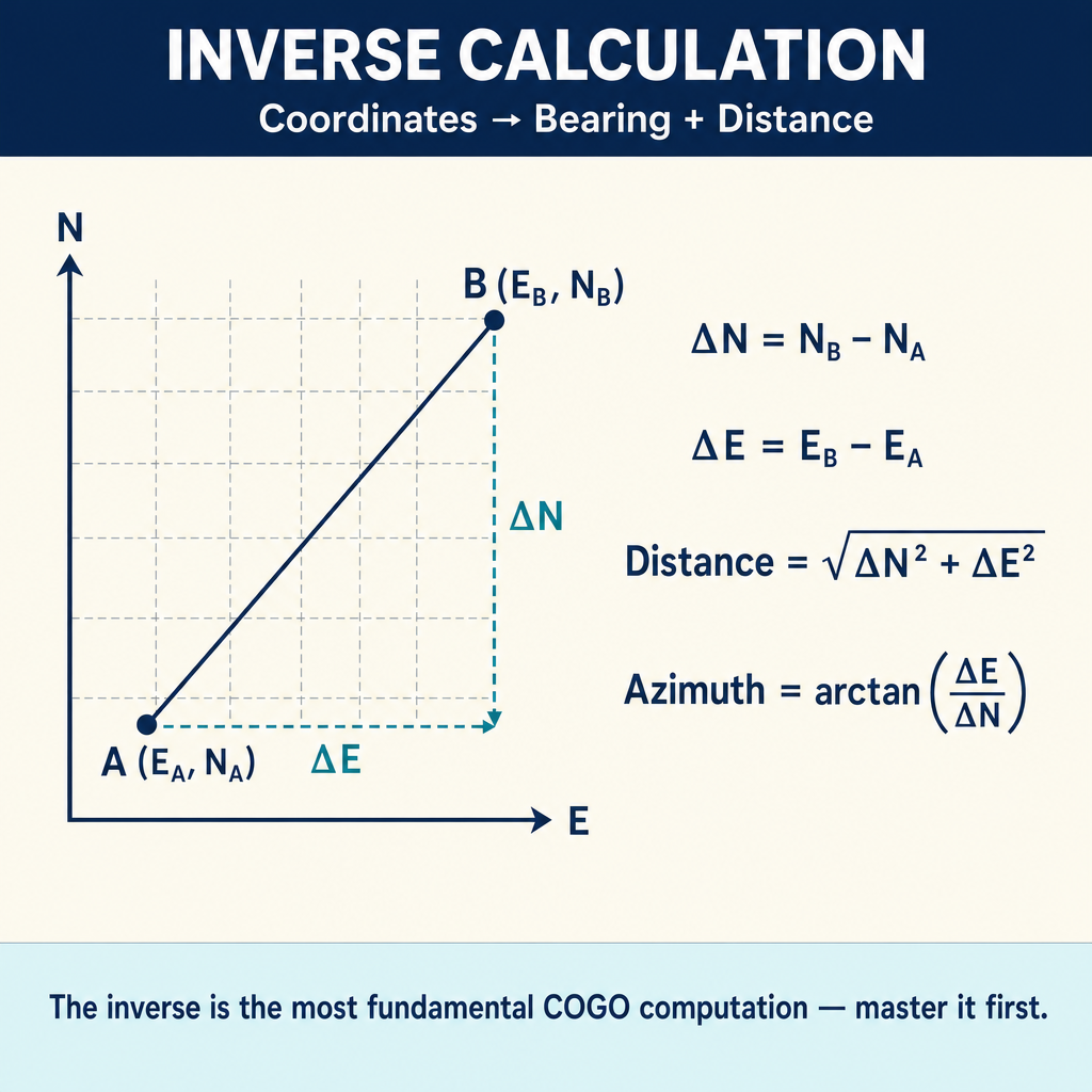
Figure PS.2.27 — COGO inverse: distance and azimuth between two points

Given the coordinates of two points, compute the distance and bearing between them.

Given: Point A (NA, EA) and Point B (NB, EB)

Delta N = NB - NA
Delta E = EB - EA
Distance = square root of (Delta N squared + Delta E squared)
Reference angle: theta = arctan(|Delta E| / |Delta N|), always in [0, 90 degrees]
Azimuth = theta combined with the quadrant per the table below

Quadrant rules for azimuth:

Delta N	Delta E	Quadrant	Azimuth
+	+	NE (I)	theta
-	+	SE (II)	180 - theta
-	-	SW (III)	180 + theta
+	-	NW (IV)	360 - theta

Always take the arctan of the absolute values of dE and dN so theta is in [0, 90]. If you use the signed arctan(dE/dN) directly, your calculator returns a result in [-90, 90] only — meaning the SE and NW quadrants come back wrong without adjustment. The software function atan2(dE, dN) returns the azimuth directly without needing this table.

Traverse (Forward Computation)

Given a starting point, bearing, and distance, compute the endpoint coordinates.

Given: Point A (NA, EA), azimuth, distance

Delta N = distance x cosine(azimuth)
Delta E = distance x sine(azimuth)
NB = NA + Delta N
EB = EA + Delta E

Bearing-Bearing Intersection

Given two points with known coordinates and a bearing from each, find their intersection point. This is solved by establishing the two line equations from the points and bearings, then solving the system simultaneously.

Bearing-Distance Intersection

Given a point with a known bearing and another point with a known distance, find their intersection. This produces two possible solutions; the surveyor must determine which is correct based on field evidence or geometric context.

Distance-Distance Intersection

Given two points with known distances to an unknown point, find the intersection. This also produces two solutions (the unknown point lies on one of two locations where the distance circles intersect).

Traverse Adjustment

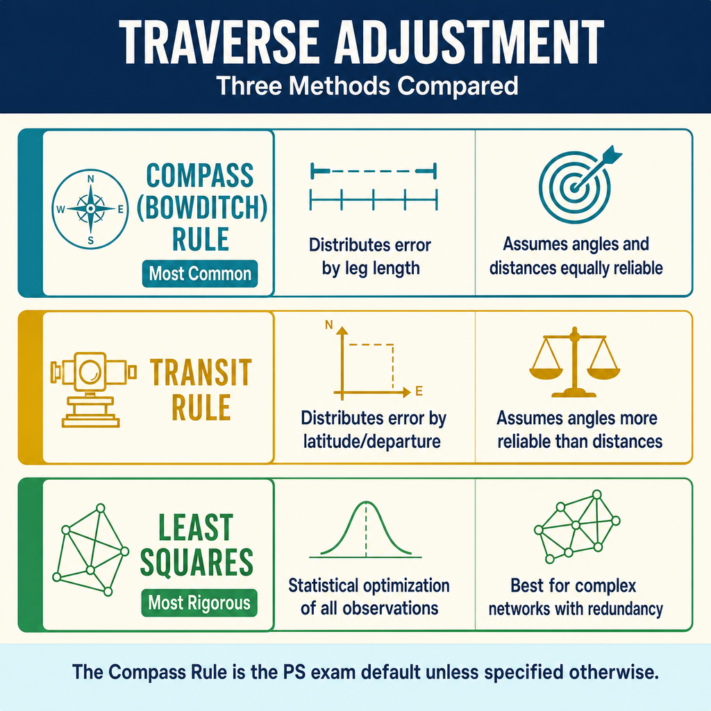
Figure PS.2.28 — Compass / Transit / Least Squares adjustment methods

After computing raw traverse coordinates, the misclosure is distributed among the traverse courses using an adjustment method. The choice of method depends on the accuracy requirements and the characteristics of the survey.

Compass Rule (Bowditch Method)

The compass rule distributes the linear misclosure in proportion to the length of each course. It assumes that angular and distance measurements are equally reliable.

Correction for each course:

Correction in N = -(total misclosure in N) x (course length / total traverse perimeter)
Correction in E = -(total misclosure in E) x (course length / total traverse perimeter)

The compass rule is the most widely used method for boundary and land surveys. It is simple, intuitive, and produces reasonable results when angular and distance accuracies are comparable.

Transit Rule

The transit rule distributes the misclosure in proportion to the absolute values of the latitude and departure of each course.

Correction for each course:

Correction in N = -(total misclosure in N) x (absolute Delta N of course / sum of all absolute Delta N values)
Correction in E = -(total misclosure in E) x (absolute Delta E of course / sum of all absolute Delta E values)

The transit rule gives slightly different results than the compass rule. It is generally considered appropriate when distance measurements are more precise than angular measurements. In practice, it is less commonly used than the compass rule.

Crandall Method

The Crandall method holds the angles fixed (after angular adjustment) and distributes the remaining linear misclosure only through adjustments to the distances. It is appropriate when angular measurements are significantly more precise than distance measurements.

Least Squares Adjustment (LSQA)

Least squares adjustment is the most rigorous method for adjusting survey observations. It simultaneously adjusts all observations (angles and distances) to find the set of coordinates that minimizes the sum of the squared residuals, weighted by the estimated precision of each observation.

Advantages of least squares over rule-based methods:

Feature	Compass/Transit Rule	Least Squares
Weights observations	No (implicit equal weight)	Yes (based on estimated precision)
Statistical output	No	Provides residuals, error ellipses, confidence intervals
Handles redundancy	Limited	Fully exploits all redundant observations
Detects blunders	Limited	Statistical testing of residuals
Network adjustment	Not applicable	Handles complex networks with multiple loops
Rigorous	No	Mathematically rigorous

Observation equations express each measurement as a function of the unknown coordinates plus a residual:

For a distance observation: computed distance (from adjusted coordinates) = observed distance + residual
For an angle observation: computed angle (from adjusted coordinates) = observed angle + residual

The adjustment minimizes the weighted sum of squared residuals.

Weight matrix assigns weights to observations inversely proportional to their variance. More precise measurements receive higher weights and have more influence on the adjusted coordinates.

Output statistics from least squares adjustment include:

Adjusted coordinates and their standard deviations
Error ellipses showing the shape and orientation of position uncertainty
Residuals for each observation (helping identify blunders)
Chi-square test for overall model validity
Relative error ellipses between points

Area Computations

Coordinate Method

The area of a polygon defined by coordinate vertices is computed using the coordinate method (also called the shoelace formula or surveyor's formula):

Area = one-half of the absolute value of the sum of (Ni x Ei+1 - Ni+1 x Ei)

where the summation goes around the polygon, with the last point connected back to the first.

This is the standard method for computing areas from coordinate data. It works for any polygon shape, including irregular boundaries.

Double Meridian Distance (DMD) Method

The DMD method computes area from the latitudes and departures of each course. The double meridian distance of a course is defined as twice the perpendicular distance from the midpoint of the course to a reference meridian (typically the meridian through the most westerly point).

DMD rules:

DMD of the first course = departure of the first course
DMD of any subsequent course = DMD of the preceding course + departure of the preceding course + departure of the current course
DMD of the last course should equal the negative of its departure (a check)

Double area = sum of (DMD of each course x latitude of that course)

Area = absolute value of double area divided by 2

Double Parallel Distance (DPD) Method

The DPD method is analogous to DMD but uses distances parallel to the east-west axis rather than the north-south axis. It produces the same result and serves as a computational check.

Horizontal Curves

Horizontal curves connect straight-line (tangent) sections of roads, boundaries, and other linear features. The most common type is the simple circular curve.

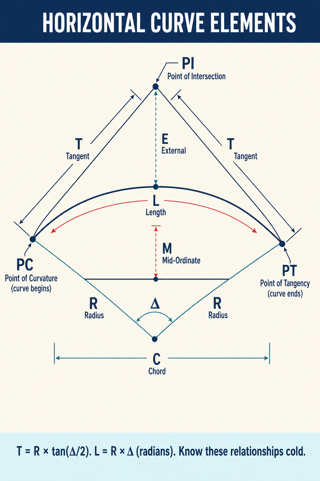
Figure PS.2.29 — Horizontal curve elements diagram

Circular Curve Elements

Element	Symbol	Definition
Radius	R	Radius of the circular arc
Degree of curve	D	Central angle subtended by a 100-foot arc (arc definition) or chord
Delta (central angle)	Delta	Angle of deflection between tangents
Tangent length	T	Distance from PI to PC or PT
Length of curve	L	Arc length from PC to PT
Long chord	LC	Straight-line distance from PC to PT
External distance	E	Distance from PI to midpoint of curve
Middle ordinate	M	Distance from midpoint of curve to midpoint of long chord
Point of curvature	PC	Beginning of curve
Point of intersection	PI	Intersection of tangents
Point of tangency	PT	End of curve

Key Formulas

T = R x tangent(Delta/2)
L = R x Delta (in radians), or L = (Delta/D) x 100 for arc definition
LC = 2R x sine(Delta/2)
E = R x (secant(Delta/2) - 1), which equals R x (1/cosine(Delta/2) - 1)
M = R x (1 - cosine(Delta/2))
D = 5729.578 / R (arc definition, feet)

Curve Stationing

Stationing along a curve is measured along the arc. Points on the curve are located by:

Computing the deflection angle from the PC to the desired point
Deflection angle = (arc length from PC to point) / (2R) in radians, converted to degrees
The chord distance from PC to the point = 2R x sine(deflection angle)

Vertical Curves

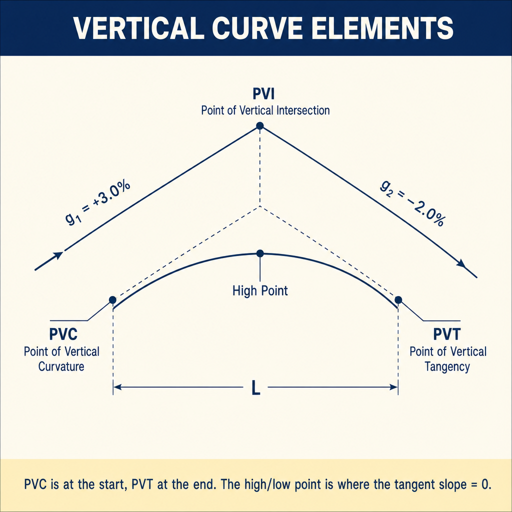
Figure PS.2.30 — Vertical crest curve with high point

Vertical curves provide smooth transitions between different grades in roadway profiles. The standard vertical curve is a parabola.

Key Elements

Element	Definition
PVC (or BVC)	Point of vertical curvature (beginning)
PVI	Point of vertical intersection
PVT (or EVC)	Point of vertical tangency (end)
L	Length of vertical curve
g1	Grade of incoming tangent (percent)
g2	Grade of outgoing tangent (percent)
A	Algebraic difference of grades: A = g2 - g1
K	Rate of vertical curvature: K = L / A

Elevation Computation

The elevation at any point on a vertical curve is computed using:

Elevation = elevation at PVC + g1 x x + (A / (2L)) x x squared

where x is the horizontal distance from the PVC.

High/low point of a vertical curve occurs at horizontal distance: x = -g1 × L / A from the PVC (valid when the computed x falls between 0 and L, indicating a turning point exists within the curve).

Coordinate Transformations

Coordinate transformations convert positions between different coordinate systems. Common transformations in surveying include:

Two-Dimensional Conformal (Helmert) Transformation

Converts between two 2D coordinate systems using four parameters: two translations, one rotation, and one scale factor. Requires a minimum of two common points.

Affine Transformation

Uses six parameters: two translations, two scales, two rotations (or equivalently, rotation plus shear). Requires a minimum of three common points. More flexible than conformal but does not preserve shape.

Three-Dimensional Transformation (Seven-Parameter)

Converts between two 3D coordinate systems using three translations, three rotations, and one scale factor. Used for datum transformations between different geodetic reference frames.

Missing Line and Area Computations

Professional surveyors frequently encounter incomplete boundary descriptions that require computation of missing elements:

Missing bearing and distance of one course in a closed traverse (computed from the misclosure of the remaining courses)
Missing bearings of two courses (with all distances known)
Missing distances of two courses (with all bearings known)
Cutoff line computations for dividing parcels into specified areas

These problems are solved using the coordinate equations for each unknown course and the closure conditions of the polygon.

Common wrong path — trusting a single-course missing-line result without verification. When one bearing and distance are missing from an otherwise closed traverse, the missing course can be computed exactly from the sum of the known courses — its bearing and distance come out as if by magic. But this magic assumes all the other courses are correct. If one of the "known" courses has a blunder (wrong bearing, transposed digits), the computed missing course will absorb that error exactly — it will close the traverse mathematically but place the missing line in the wrong position. The result looks clean (closure is perfect by construction) but is wrong in the real world. Exam questions bait this by giving a traverse with a plausible blunder hidden in a "known" course and asking for the missing line; the computed answer will satisfy closure but not match any reasonable real-world interpretation. Always sanity-check a computed missing line against map evidence, adjoiner deeds, and field conditions — do not treat a mathematical solution as a physical truth.

Quick retrieval check — try before reading on.

▶A closed traverse has five courses. Four are fully described; the fifth (the missing course) is computed from the closure condition to be N 85° 00' E, 145.20 ft. You plot the full traverse on a map and notice that the fifth course aligns with a chain-link fence the client has mentioned. On the ground, you measure the fifth course directly as N 72° 30' E, 138.80 ft. What is the most likely explanation?

One or more of the other four courses likely contains a blunder. The computed missing line closed the traverse mathematically, but because it was derived from the assumption that the four known courses were correct, any error in them propagated entirely into the computed course. The ground measurement (N 72°30' E, 138.80 ft) is almost certainly closer to the truth — especially since it aligns with physical fence evidence. Next steps:

Re-examine each of the four "known" courses for typos, transposed digits, or reversed bearings.
Compare adjoiner deeds to check whether any of the four courses should be different.
Recompute the missing line with each suspected correction until both (a) the traverse closes and (b) the computed fifth course matches the field measurement.

This is why missing-line computations should never be accepted blindly — the math is exact, but it only repairs the consequence of the blunder, not the cause. Treat a large discrepancy between the computed missing line and the measured value as evidence of a blunder elsewhere in the traverse, not as an error in your measurement.

Exam Tips

The compass (Bowditch) rule distributes misclosure in proportion to course length -- this is the most commonly tested adjustment method
For area computation by coordinates, the shoelace formula is the standard approach
In horizontal curve computations, T = R x tan(Delta/2) and L = R x Delta (radians) are the most frequently needed formulas
Least squares adjustment provides statistical quality measures that rule-based methods cannot
The high/low point of a vertical curve is found at x = -g1 x L / A from the PVC
DMD of the first course equals the departure of the first course
Two-dimensional conformal transformation requires two common points minimum
Missing line problems in a closed traverse are solved from the closure condition