FS Exam Preparation

Comprehensive preparation for the Fundamentals of Surveying (FS) exam. 7 modules covering all 7 exam domains with 60 in-depth topics.

Progress0/60

Lesson 5

Control Surveys & Standards

Learning Objectives

After completing this topic, you should be able to:

Define horizontal and vertical control and their purposes
Describe the national accuracy standards for geodetic control
Design a basic control network
Explain the concept of order, class, and accuracy
Calculate positional accuracy from network adjustments
Understand the role of the National Spatial Reference System (NSRS)

Overview

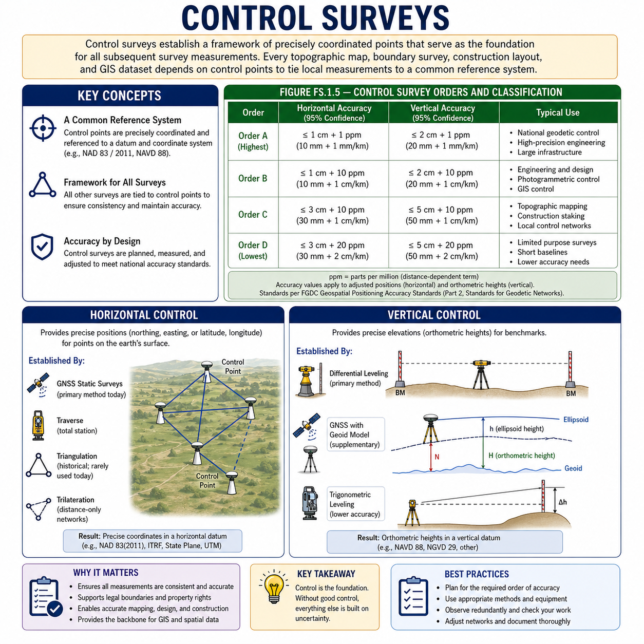
Control surveys establish a framework of precisely coordinated points that serve as the foundation for all subsequent survey measurements. Every topographic map, boundary survey, construction layout, and GIS dataset depends on control points to tie local measurements to a common reference system.

The quality of control surveys is defined by national accuracy standards published by the Federal Geographic Data Committee (FGDC). Understanding these standards -- and how to meet them -- is essential for the FS exam and professional practice.

Key Concepts

Figure FS.1.5 — Control surveys: framework, horizontal vs vertical control, accuracy by order, and how each is established

Horizontal vs. Vertical Control

Horizontal control provides precise positions (northing, easting, or latitude, longitude) for points on the earth's surface. Horizontal control networks are established by:

GNSS static surveys (primary method today)
Traverse (total station)
Triangulation (historical; rarely used today)
Trilateration (distance-only networks)

Vertical control provides precise elevations (orthometric heights) for benchmarks. Vertical control is established by:

Differential leveling (primary method)
GNSS with geoid model (supplementary)
Trigonometric leveling (lower accuracy)

The National Spatial Reference System (NSRS)

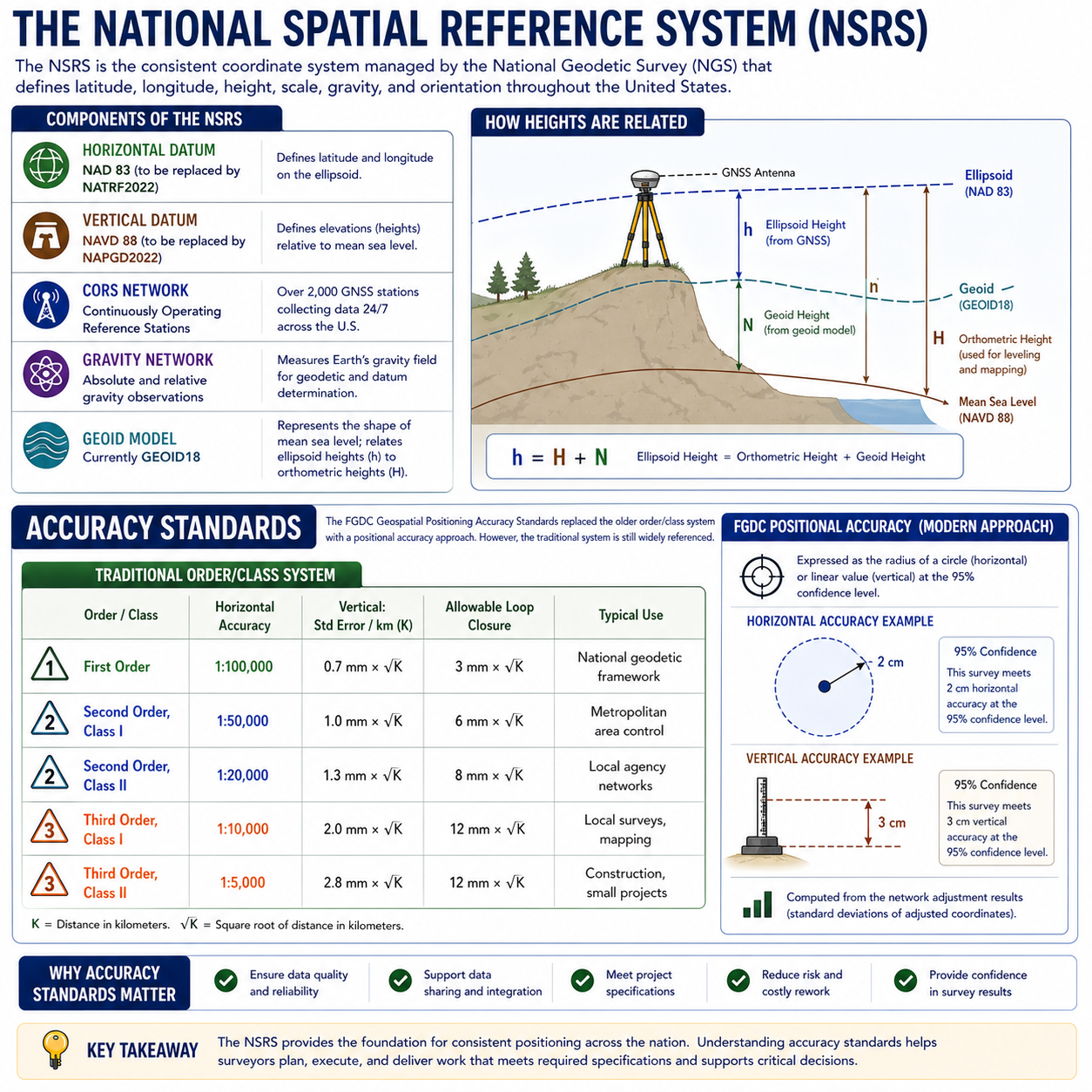
Figure FS.1.5c — The NSRS: NAD 83 / NAVD 88 datums, CORS, gravity, GEOID18; ellipsoid vs geoid vs orthometric heights; FGDC accuracy standards

The NSRS is the consistent coordinate system managed by the National Geodetic Survey (NGS) that defines latitude, longitude, height, scale, gravity, and orientation throughout the United States.

Components of the NSRS:

Horizontal datum: NAD 83 (to be replaced by the North American Terrestrial Reference Frame, NATRF2022)
Vertical datum: NAVD 88 (to be replaced by the North American-Pacific Geopotential Datum, NAPGD2022)
CORS network: Continuously Operating Reference Stations
Gravity network: Absolute and relative gravity observations
Geoid model: Currently GEOID18; relates ellipsoid heights to orthometric heights

Accuracy Standards

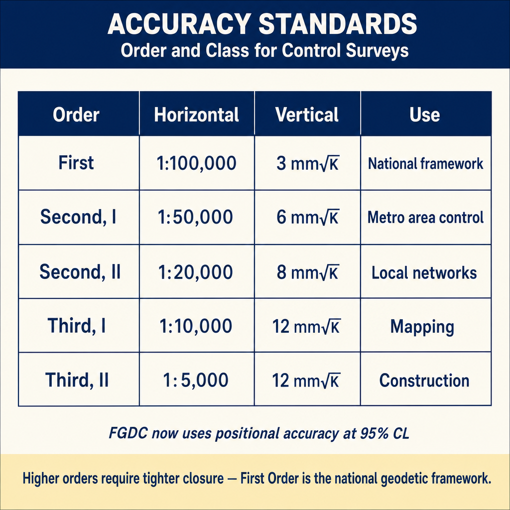
Figure FS.1.5f — FGCS accuracy standards by order (1st, 2nd I/II, 3rd I/II)

The FGDC Geospatial Positioning Accuracy Standards replaced the older order/class system with a positional accuracy approach. However, the traditional system is still widely referenced.

Traditional Order/Class System (1984 FGCS):

The horizontal and vertical networks classify differently — they are NOT a single combined order/class system. Horizontal First Order is not subdivided into classes; vertical Third Order is not subdivided into classes either.

Horizontal accuracy (per Ghilani Table 19.4):

Order / Class	Relative-Distance Accuracy	Typical Use
First Order	1:100,000	National geodetic framework
Second Order, Class I	1:50,000	Metropolitan area control
Second Order, Class II	1:20,000	Local agency networks
Third Order, Class I	1:10,000	Local surveys, mapping
Third Order, Class II	1:5,000	Construction, small projects

Vertical accuracy (per Ghilani Table 19.5):

Order / Class	Std Error per km	Allowable Loop Closure
First Order, Class I	0.5 mm × √K	4 mm × √K
First Order, Class II	0.7 mm × √K	5 mm × √K
Second Order, Class I	1.0 mm × √K	6 mm × √K
Second Order, Class II	1.3 mm × √K	8 mm × √K
Third Order	2.0 mm × √K	12 mm × √K

Loop misclosure values are from FGCS Section 5.5 (Ghilani 13e). For First Order Class I, the section (one-way) constant is 3 mm × √K; the other classes use the same constants for sections and loops.

FGDC Positional Accuracy:

Expressed as the radius of a circle (horizontal) or linear value (vertical) at the 95% confidence level
Example: "This survey meets 2 cm horizontal accuracy at 95% confidence"
Computed from the network adjustment results (standard deviations of adjusted coordinates)

Network Design Principles

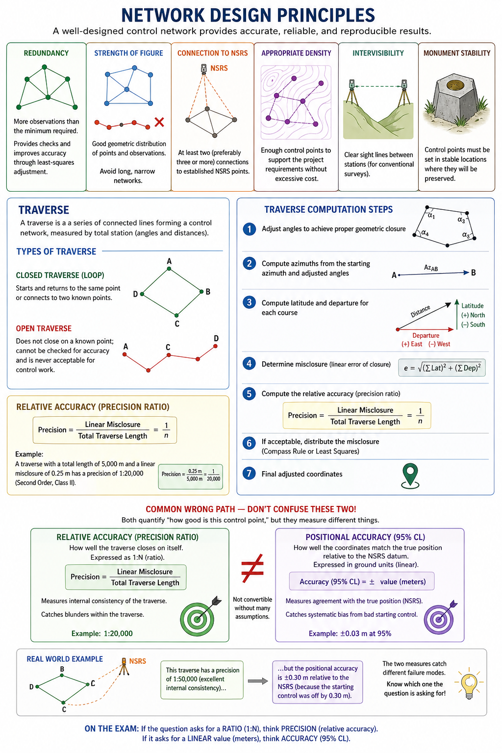
Figure FS.1.5d — Network design principles (redundancy, strength of figure, NSRS connection, density, intervisibility, monument stability) and traverse computation steps

A well-designed control network should have:

Redundancy -- More observations than the minimum required, providing checks and improving accuracy through least-squares adjustment
Strength of figure -- Good geometric distribution of points and observations; avoid long, narrow networks
Connection to NSRS -- At least two (preferably three or more) connections to established NSRS points
Appropriate density -- Enough control points to support the project requirements without excessive cost
Intervisibility (for conventional surveys) -- Clear sight lines between stations
Monument stability -- Control points must be set in stable locations where they will be preserved

Traverse

A traverse is a series of connected lines forming a control network, measured by total station (angles and distances).

Types of traverse:

Closed traverse (loop): Starts and returns to the same point or connects to two known points
Open traverse: Does not close on a known point; cannot be checked for accuracy and is never acceptable for control work

Traverse computation steps:

Adjust angles to achieve proper geometric closure
Compute azimuths from the starting azimuth and adjusted angles
Compute latitude and departure for each course
Determine misclosure (linear error of closure)
Compute the relative accuracy (ratio of linear misclosure to total traverse length)
If acceptable, distribute the misclosure (Compass Rule or Least Squares)

Relative accuracy (precision ratio):

$\text{Precision} = \frac{\text{Linear Misclosure}}{\text{Total Traverse Length}} = \frac{1}{n}$

Example: A traverse with a total length of 5,000 m and a linear misclosure of 0.25 m has a precision of 1:20,000 (Second Order, Class II).

Common wrong path — treating relative accuracy and positional accuracy as interchangeable. Both quantify "how good is this control point," but they measure different things:

Relative accuracy (precision ratio) — how well the traverse closes on itself, expressed as 1:N (e.g., 1:20,000). Measures internal consistency of the traverse.

Positional accuracy (95% CL) — how well the coordinates of a point match the true position relative to the NSRS datum, expressed in ground units (e.g., ±0.03 m at 95%).

These numbers are not convertible without making many assumptions. A traverse can have a precision ratio of 1:50,000 (excellent internal consistency) while having a positional accuracy of 0.30 m relative to the NSRS (because the starting control was off by 0.30 m). The two measures catch different failure modes: relative accuracy catches measurement blunders within the traverse; positional accuracy catches systematic bias from bad starting control. On the exam, a question that mixes the two concepts expects you to recognize which is being asked — a ratio (precision) or a linear value (accuracy). They are not the same answer to the same question.

Quick retrieval check — try before reading on.

▶A 4,000 ft closed traverse has a linear misclosure of 0.08 ft. What is the relative accuracy, and does this tell you anything about the positional accuracy of the traverse points relative to NSRS?

Relative accuracy = 0.08 / 4,000 = 1:50,000. That's excellent internal precision — the traverse closes very well, meeting First Order Class II roughly (1:50,000 standard).

But this tells you nothing about positional accuracy relative to NSRS. If the starting control point has a published positional uncertainty of 0.05 m (5 cm) in the NSRS, then every traverse point inherits at least that much positional uncertainty — the traverse cannot be more accurate in absolute terms than its starting tie. If the starting control was misidentified or has a superseded coordinate (different NAD 83 realization, for example), the positional error could be much larger. To establish positional accuracy, you need ties to multiple NSRS points and a network adjustment that reports positional standard deviations at 95% confidence. Relative accuracy and positional accuracy answer different questions, and a traverse can pass one while failing the other.

Least Squares Adjustment

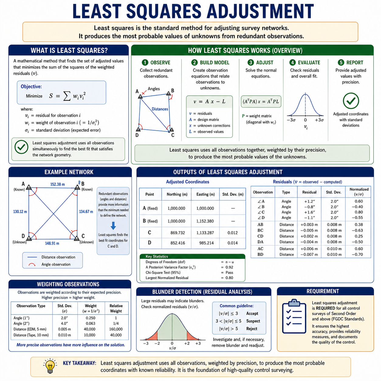
Figure FS.1.5e — Least squares adjustment: how it works, example network, weighting observations, residuals, blunder detection, FGDC requirement for second-order and above control

Least squares is the standard method for adjusting survey networks. It:

Simultaneously adjusts all observations to achieve the best fit
Weights observations according to their expected precision
Produces adjusted coordinates with standard deviations (error estimates)
Identifies blunders through residual analysis
Is required for all control surveys of Second Order and above

The FS exam may test your understanding of the concept, not the computation details of least squares.

Exam Tips

An open traverse provides no check on accuracy and is unacceptable for control work
The Compass Rule distributes misclosure proportionally to course length; it assumes equal angular and distance accuracy
Precision ratio is linear misclosure divided by total traverse length -- express it as a ratio (1:X)
Least squares adjustment is the standard for modern control surveys; it produces accuracy estimates for every point
The NSRS provides the national reference framework; all local surveys should tie to it
Know the difference between relative accuracy (precision ratio) and positional accuracy (95% confidence)
Vertical control standards use the formula C x sqrt(K), where K is the leveling distance in km
GNSS static surveys have largely replaced triangulation and trilateration for establishing horizontal control
The FS exam may give you traverse data and ask you to compute the precision ratio

FS Exam Preparation

Module 1: Surveying Processes & Methods

Module 2: Mapping Processes & Methods

Module 3: Boundary Law & Real Property

Module 4: Surveying Principles & Geodesy

Module 5: Survey Computations

Module 6: Business Concepts

Module 7: Applied Math & Statistics