Linear Algebra & Matrices

Learning Objectives

After completing this topic, you should be able to:

• Perform basic matrix operations (addition, multiplication, transpose)
• Compute the determinant of a 2x2 and 3x3 matrix
• Find the inverse of a 2x2 matrix
• Solve systems of linear equations using matrices
• Recognize the role of matrices in least squares adjustment

Overview

Linear algebra provides the mathematical framework for solving systems of equations that arise throughout surveying -- from coordinate transformations to least squares adjustments to network analysis. While the FS exam does not require advanced matrix theory, you must be able to perform basic matrix operations, solve small systems of equations, and understand how matrices are used in surveying applications.

---

Key Concepts

Matrix Basics

A matrix is a rectangular array of numbers arranged in rows and columns. An m x n matrix has m rows and n columns.

Example: A 2x3 matrix:

	Col 1	Col 2	Col 3
Row 1	3	1	4
Row 2	2	5	6

Key matrix types:

• Square matrix: Same number of rows and columns (e.g., 3x3)
• Identity matrix (I): Square matrix with 1s on the diagonal and 0s elsewhere
• Diagonal matrix: Non-zero elements only on the diagonal
• Symmetric matrix: Equal to its transpose (A = A^T)
• Vector: A matrix with one column (column vector) or one row (row vector)

Matrix Operations

Addition/Subtraction: Matrices must be the same size. Add or subtract corresponding elements.

Scalar multiplication: Multiply every element by the scalar.

Matrix multiplication (A * B):

• The number of columns in A must equal the number of rows in B
• If A is m x n and B is n x p, the result is m x p
• Element (i,j) of the result = sum of (row i of A) * (column j of B)

Example: For 2x2 matrices:

A = [a b; c d], B = [e f; g h]

A * B = [(ae+bg) (af+bh); (ce+dg) (cf+dh)]

Important: Matrix multiplication is NOT commutative: A * B does not generally equal B * A.

Transpose (A^T): Swap rows and columns. Element (i,j) becomes element (j,i).

Determinant

The determinant is a scalar value computed from a square matrix. It indicates whether the matrix is invertible (det != 0) or singular (det = 0).

2x2 determinant:

det([a b; c d]) = ad - bc

3x3 determinant (expansion along the first row):

det([a b c; d e f; g h i]) = a(ei - fh) - b(di - fg) + c(dh - eg)

Matrix Inverse

The inverse of a square matrix A, denoted A^(-1), satisfies: A * A^(-1) = I

2x2 inverse:

If A = [a b; c d], then:

A^(-1) = (1 / det(A)) * [d -b; -c a]

The inverse exists only if det(A) != 0.

Example: A = [4 3; 2 1]

det(A) = 41 - 32 = -2

A^(-1) = (1/-2) * [1 -3; -2 4] = [-0.5 1.5; 1 -2]

Solving Systems of Linear Equations

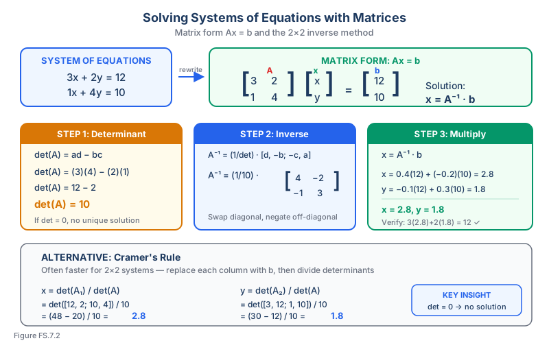
A system of linear equations can be written in matrix form: Ax = b

Where:

• A = coefficient matrix
• x = vector of unknowns
• b = vector of constants

Solution: x = A^(-1) * b

Example: Solve: 3x + 2y = 12 and x + 4y = 10

A = [3 2; 1 4], b = [12; 10]

det(A) = 34 - 21 = 10

A^(-1) = (1/10) * [4 -2; -1 3] = [0.4 -0.2; -0.1 0.3]

x = [0.4 -0.2; -0.1 0.3] * [12; 10] = [0.4*12 + (-0.2)*10; (-0.1)12 + 0.310]

x = [4.8 - 2.0; -1.2 + 3.0] = [2.8; 1.8]

Verification: 3(2.8) + 2(1.8) = 8.4 + 3.6 = 12. Correct.

Cramer's Rule

For a system Ax = b, each unknown can be found by:

x_i = det(A_i) / det(A)

Where A_i is the matrix A with column i replaced by vector b.

Example: Same system as above:

x = det([12 2; 10 4]) / det([3 2; 1 4]) = (48-20) / 10 = 28/10 = 2.8

y = det([3 12; 1 10]) / det([3 2; 1 4]) = (30-12) / 10 = 18/10 = 1.8

Common wrong path — matrix multiplication order. Matrix multiplication is not commutative: A × B generally does NOT equal B × A. Students routinely get this wrong under time pressure, especially when setting up coordinate transformations. The dimensions also have to line up: A (m × n) × B (n × p) gives an (m × p) result — but B × A may not even be defined if p ≠ m. In surveying, this matters for coordinate transformation: the correct order is transformation matrix × coordinate vector, producing the transformed coordinate vector. Reversing the order either gives the wrong answer or is mathematically undefined. Exam questions test this by presenting two matrices that are dimension-compatible in one order but not the other; the answer requires you to identify the correct order.

Quick retrieval check — try before reading on.

▶Given A = [[2, 1], [3, 4]] and B = [[1, 0], [2, 5]], compute both A×B and B×A. Are they equal?

A × B:

• Row 1: [(2)(1) + (1)(2), (2)(0) + (1)(5)] = [4, 5]
• Row 2: [(3)(1) + (4)(2), (3)(0) + (4)(5)] = [11, 20]
• Result: [[4, 5], [11, 20]]

B × A:

• Row 1: [(1)(2) + (0)(3), (1)(1) + (0)(4)] = [2, 1]
• Row 2: [(2)(2) + (5)(3), (2)(1) + (5)(4)] = [19, 22]
• Result: [[2, 1], [19, 22]]

Not equal. The element values differ substantially — matrix multiplication is not commutative. This is a fundamental property that students must internalize: the order of matrix multiplication changes the result. In surveying applications (coordinate transformations, least squares normal equations, covariance propagation), always apply matrices in the correct order. Dimensional check: if A is m × n and B is n × p, then A × B works (m × p result), but B × A requires p = m for B × A to be defined at all.

Application to Surveying

Matrices are used throughout surveying for:

• Least squares adjustment: The normal equations Nx = t are solved using matrices
• Coordinate transformations: The 4-parameter and 7-parameter transformations are expressed as matrix equations
• Network adjustment: Large systems of observation equations are assembled and solved as matrix problems
• Error propagation: The variance-covariance matrix describes the precision of adjusted coordinates

FS Matrix Workflow

For the FS exam, keep matrix work mechanical:

1. Write dimensions beside each matrix. This prevents invalid multiplication.
2. Check determinant before finding an inverse. If det = 0, there is no unique inverse solution.
3. Use Cramer's rule for small 2x2 systems. It is often faster and less error-prone than writing the inverse.
4. Verify the solution in the original equations. Substitution catches most arithmetic errors.
5. For transformations, keep the coordinate vector order consistent. Do not swap north/east or x/y halfway through.

Surveying Example: Transformation Setup

A 2D coordinate transformation (4-parameter conformal / Helmert form) can be written as (Ghilani, Adjustment Computations: Spatial Data Analysis, 5th Ed., Ch. 18):

N' = aN - bE + tN
E' = bN + aE + tE

[N']   [a  -b][N]   [tN]
[E'] = [b   a][E] + [tE]

The rotation/scale matrix multiplies the coordinate vector, then translations are added. Reversing that order changes the meaning of the operation. This is why matrix multiplication order is not just a math rule; it changes the resulting survey coordinates. (Coordinate-ordering convention: in surveying, N is plotted on the vertical y-axis and E on the horizontal x-axis, so this form treats N as the first coordinate. Some GIS and software libraries use (E, N) ordering instead — verify your tool's convention before applying published transformation parameters.)

---

Exam Tips

• For the FS exam, focus on 2x2 and 3x3 matrices -- larger matrices are rare
• Know how to compute a 2x2 determinant and inverse by hand -- these are fast and common
• Matrix multiplication order matters: AB != BA in general
• When solving systems of equations, Cramer's rule is often faster for 2x2 systems than computing the full inverse
• If the determinant is zero, the system has no unique solution (the equations are dependent or inconsistent)
• For 3x3 determinants, practice the cofactor expansion method until it is reliable
• The FS reference handbook provides matrix formulas, but you must know how to apply them
• On the FS exam, matrix problems typically appear as systems of equations or coordinate transformation problems, not abstract linear algebra

---

Related Test Topics

• Least Squares Adjustments (Topic 5.5)
• Coordinate Geometry (Topic 5.1)
• Error Analysis and Propagation (Topic 7.4)

---

Further Reading

Authoritative sources for deeper study

• Ghilani & Wolf, Adjustment Computations (5th Ed., 2010) — Matrix algebra, normal equations, and least squares formulation.

• Ghilani & Wolf, Adjustment Computations (5th Ed., 2010) — Authoritative treatment of least-squares adjustment for surveying networks.

---

Last updated: 2026-04-17