Probability & Statistics Fundamentals

Learning Objectives

After completing this topic, you should be able to:

• Compute the mean, median, mode, and standard deviation of a dataset
• Describe the properties of the normal distribution
• Apply the 68-95-99.7 rule (empirical rule)
• Compute confidence intervals for the mean
• Apply basic probability rules
• Interpret the t-distribution for small samples

Overview

Probability and statistics provide the framework for quantifying uncertainty in measurements. Every survey measurement contains error, and statistical methods allow the surveyor to estimate the most probable value, quantify the uncertainty, and determine whether results meet specified standards. The FS exam tests your ability to compute basic statistics, work with the normal distribution, and construct confidence intervals.

---

Key Concepts

Descriptive Statistics

Mean (arithmetic average):

x_bar = (x1 + x2 + ... + xn) / n = (Sum of xi) / n

Median: The middle value when data is sorted. For an even number of observations, average the two middle values.

Mode: The most frequently occurring value.

Range: Maximum value minus minimum value.

Measures of Dispersion

Variance (population):

sigma^2 = Sum of (xi - mu)^2 / N

Variance (sample):

s^2 = Sum of (xi - x_bar)^2 / (n - 1)

Standard deviation:

sigma = sqrt(variance) for population

s = sqrt(s^2) for sample

Why n-1? The sample variance uses (n-1) in the denominator (called Bessel's correction) because the sample mean is used instead of the true population mean, which removes one degree of freedom.

Standard deviation of the mean (standard error):

SE = s / sqrt(n)

(Equivalently denoted s_mean or s_x̄. Reserve σ for the true population standard deviation; the SE estimated from a sample uses s and is sometimes written σ̂_mean. This formula assumes the n observations are statistically independent — correlated observations require the full variance-covariance form.)

This measures how precisely the mean is known, not how variable individual measurements are.

The Normal Distribution

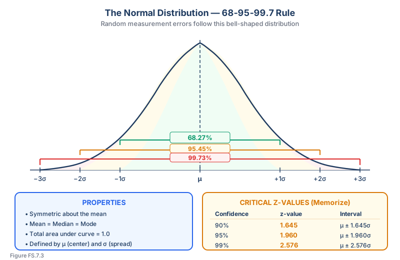
The normal (Gaussian) distribution is the bell-shaped curve that describes the distribution of random errors in measurements.

Properties:

• Symmetric about the mean
• Mean = median = mode
• Defined by two parameters: mean (mu) and standard deviation (sigma)
• Total area under the curve = 1.0

The 68-95-99.7 rule (empirical rule):

Interval	Probability
mu +/- 1 sigma	68.27%
mu +/- 2 sigma	95.45%
mu +/- 3 sigma	99.73%

In surveying terms: About 68% of measurements fall within one standard deviation of the mean, about 95% within two standard deviations, and about 99.7% within three standard deviations.

Symmetric Probability Intervals for a Single Observation

For the normal distribution, these intervals describe the spread of individual measurements drawn from N(μ, σ²). To estimate uncertainty in the mean of n observations, replace σ with σ/√n (or s/√n) — see Confidence Intervals below.

Z-values below are from the standard normal table (Ghilani & Wolf, Elementary Surveying, 13th Ed., Eqs. 3.7–3.8):

Coverage	Z-value	Interval
68.27%	1.000	mu +/- 1.000 * sigma
90%	1.645	mu +/- 1.645 * sigma
95%	1.960	mu +/- 1.960 * sigma
99%	2.576	mu +/- 2.576 * sigma
99.73%	3.000	mu +/- 3.000 * sigma

Confidence Intervals for the Mean

The confidence interval estimates the range within which the true population mean likely falls:

CI = x_bar +/- z * (s / sqrt(n))

Where:

• x_bar = sample mean
• z = z-value for the desired confidence level
• s = sample standard deviation
• n = number of observations

Example: 10 measurements of a distance yield a mean of 325.42 ft with s = 0.08 ft. Find the 95% confidence interval.

CI = 325.42 +/- 1.960 * (0.08 / sqrt(10))

CI = 325.42 +/- 1.960 * 0.0253

CI = 325.42 +/- 0.05 ft

CI = (325.37, 325.47) ft

The t-Distribution

For small samples (n < 30), the normal distribution underestimates the uncertainty. The t-distribution accounts for the additional uncertainty from estimating the standard deviation from a small sample.

CI = x_bar +/- t_(alpha/2, n-1) * (s / sqrt(n))

The t-value depends on:

• The desired confidence level (alpha)
• The degrees of freedom (n - 1)

As n increases, the t-distribution approaches the normal distribution. For n > 30, the difference is negligible.

Common wrong path — confusing standard deviation with standard error. These two quantities both describe "uncertainty" but measure different things:

• Standard deviation (s) — spread of individual measurements around the mean. Describes how variable the raw data is.
• Standard error of the mean (s/√n) — uncertainty of the average. Describes how well you know the true mean.

The two are related by a factor of √n, which for 10 measurements is ~3.2 and for 100 measurements is 10. Students sometimes build confidence intervals using s instead of s/√n, producing intervals that are √n times too wide — making every measurement appear far more uncertain than it is. On the exam, the formula $\bar{x} \pm z \cdot s/\sqrt{n}$ (confidence interval for the mean) uses the standard error, not the standard deviation. $\bar{x} \pm z \cdot s$ would describe the interval containing ~95% of individual observations, not the interval containing the true mean.

Quick retrieval check — try before reading on.

▶25 repeated observations of an angle yield a mean of 45° 12' 30" with a sample standard deviation of 8". Compute the 95% confidence interval for the mean angle. How does your answer compare to 45° 12' 30" ± 8"?

Standard error = $s/\sqrt{n} = 8"/\sqrt{25} = 8"/5 = 1.6"$.

95% CI = $\bar{x} \pm 1.960 \times \text{SE} = 45° 12' 30" \pm 1.960 \times 1.6" = 45° 12' 30" \pm \mathbf{3.14"}$.

The interval $\bar{x} \pm 8"$ (about $\bar{x} \pm s$) would describe the range containing ~68% of individual observations — not the confidence interval for the mean. The mean of 25 observations is known to within ~3.14 seconds at 95% confidence, while individual observations span ±8 seconds at 1σ (68% band). Increasing n from 25 to 100 would reduce the SE from 1.6" to 0.8", tightening the 95% CI to ±1.57". This is why long-duration static GNSS sessions produce much smaller positioning uncertainty than RTK — more observations → smaller SE → tighter interval.

Basic Probability Rules

Addition rule: P(A or B) = P(A) + P(B) - P(A and B)

Multiplication rule (independent events): P(A and B) = P(A) * P(B)

Complement rule: P(not A) = 1 - P(A)

Surveying Interpretation

Statistics questions on the FS exam are usually about measurement uncertainty, not abstract probability. Translate each statistic into field meaning:

Statistic	Surveying meaning
Mean	Best estimate from repeated observations
Standard deviation	Scatter of individual observations
Standard error	Uncertainty of the mean
Confidence interval	Range likely to contain the true value
Outlier	Observation that may be a blunder or rare random error

If a problem asks whether more observations improve precision, the answer usually depends on the standard error: increasing n reduces s/sqrt(n), but it does not automatically remove systematic error or blunders.

Mini Drill: Standard Error

Nine repeated distance observations have sample standard deviation s = 0.030 ft. What is the standard error of the mean?

SE = s / sqrt(n) = 0.030 / sqrt(9) = 0.030 / 3 = 0.010 ft.

The individual observations scatter by about 0.030 ft, but the average is known to about 0.010 ft at one standard error. This distinction is a favorite FS trap.

---

Exam Tips

• Always use (n-1) in the denominator for sample standard deviation -- the FS exam almost always deals with samples, not populations
• The standard deviation of the mean = s / sqrt(n) -- this is how precision improves with more measurements
• Memorize the z-values: 1.645 (90%), 1.960 (95%), 2.576 (99%)
• Use the t-distribution for small samples (n < 30) when the exam provides a t-table
• The 68-95-99.7 rule is an approximation for the normal distribution; exact values differ slightly (95.45% vs. 95%)
• Confidence interval gets narrower as: (1) n increases, (2) s decreases, or (3) confidence level decreases
• The FS exam reference handbook includes z-tables and t-tables -- know how to read them
• Mean, median, and mode are equal for a normal distribution; if they differ significantly, the data may not be normally distributed

---

Related Test Topics

• Error Analysis and Propagation (Topic 7.4)
• Measurement Accuracy and Precision (Topic 7.5)
• Data Analysis and Quality Control (Topic 7.6)
• Least Squares Adjustments (Topic 5.5)

---

Further Reading

Authoritative sources for deeper study

• Ghilani & Wolf, Adjustment Computations (5th Ed., 2010), Ch. 3 — Statistical foundations: mean, variance, distributions, confidence.

• Ghilani & Wolf, Adjustment Computations (5th Ed., 2010) — Authoritative treatment of least-squares adjustment for surveying networks.

• FGDC Geospatial Positioning Accuracy Standards — National standard for positional accuracy reporting (NSSDA).

---

Last updated: 2026-04-17