Measurement Accuracy & Precision

Learning Objectives

After completing this topic, you should be able to:

• Define and distinguish between accuracy and precision
• Explain significant figures and rounding rules
• Describe measurement standards and their accuracy classifications
• Compute and interpret the most probable value of a measurement
• Apply the concept of least count to measurement instruments
• Relate measurement quality to survey specifications

Overview

Accuracy and precision are the two fundamental measures of measurement quality. Every surveyor must understand the distinction, know how to quantify each, and be able to determine whether a set of measurements meets a given specification. The FS exam tests these concepts both as definitions and in applied problems where you must evaluate measurement quality.

---

Key Concepts

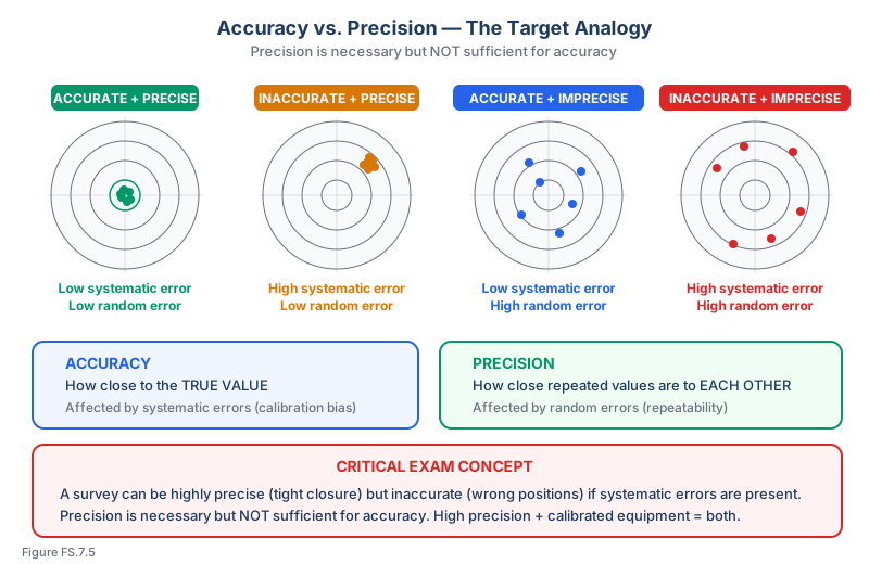
Accuracy vs. Precision

Accuracy: How close a measurement is to the true value (correctness).

Precision: How close repeated measurements are to each other (repeatability).

Scenario	Accurate?	Precise?	Analogy
Measurements cluster around the true value	Yes	Yes	Shots grouped at the bullseye
Measurements cluster tightly but away from true value	No	Yes	Shots grouped but off-center
Measurements scattered around the true value	Yes (on average)	No	Shots scattered around the bullseye
Measurements scattered away from the true value	No	No	Shots scattered and off-center

Key insight: Precision is necessary but NOT sufficient for accuracy. A precise but inaccurate result indicates systematic error. A precise and accurate result indicates both low systematic and low random error.

Most Probable Value

The most probable value (MPV) of a measured quantity is the value most likely to be correct given the available measurements. For equally weighted measurements, the MPV is the arithmetic mean.

For unequally weighted measurements, the MPV is the weighted mean:

MPV = Sum(wi * xi) / Sum(wi)

Where wi is the weight assigned to measurement i.

Residual: The difference between an individual measurement and the MPV:

vi = xi - MPV

The sum of residuals should be approximately zero (exactly zero for equally weighted measurements).

Significant Figures

Significant figures indicate the precision of a measurement:

Rules for counting significant figures:

1. All nonzero digits are significant: 345.6 has 4 significant figures
2. Zeros between nonzero digits are significant: 3006 has 4 significant figures
3. Leading zeros are NOT significant: 0.0045 has 2 significant figures
4. Trailing zeros after a decimal point ARE significant: 3.450 has 4 significant figures
5. Trailing zeros in a whole number are ambiguous: 3400 could have 2, 3, or 4 significant figures (use scientific notation to clarify: 3.400 x 10^3 has 4)

Rules for computations:

• Addition/subtraction: Result has the same number of decimal places as the least precise input
• Multiplication/division: Result has the same number of significant figures as the input with the fewest

Instrument Resolution and Least Count

The least count is the smallest division that can be read on a measuring instrument. It sets the minimum resolution of the measurement:

Instrument	Typical Least Count
Engineer's tape (ft)	0.01 ft
Metric tape	1 mm (0.001 m)
Level rod	0.001 ft or 1 mm
Total station (angle)	1" to 5"
Total station (distance)	1 mm + 1 ppm
GNSS (RTK)	10-20 mm horizontal

Estimation between divisions: An experienced observer can typically estimate to 1/10 of the least count. For example, a level rod with 0.01 ft divisions can be estimated to 0.001 ft.

Measurement Standards and Classifications

Survey accuracy is specified by national standards:

FGCS (Federal Geodetic Control Subcommittee) Standards (1984):

The horizontal and vertical networks classify differently — they are NOT a single combined order/class system. Horizontal First Order is not subdivided into classes; vertical Third Order is not subdivided into classes either.

Horizontal accuracy (per Ghilani Table 19.4):

Order / Class	Relative-Distance Accuracy
First Order	1:100,000
Second Order, Class I	1:50,000
Second Order, Class II	1:20,000
Third Order, Class I	1:10,000
Third Order, Class II	1:5,000

Vertical accuracy (per Ghilani Table 19.5):

Order / Class	Std Error per km	Allowable Loop Closure
First Order, Class I	0.5 mm × √K	4 mm × √K
First Order, Class II	0.7 mm × √K	5 mm × √K
Second Order, Class I	1.0 mm × √K	6 mm × √K
Second Order, Class II	1.3 mm × √K	8 mm × √K
Third Order	2.0 mm × √K	12 mm × √K

Where K = distance in km. The "Std Error per km" column applies to a 1-km leveling section; the "Allowable Loop Closure" column applies to a closed leveling loop. For First Order Class I the section misclosure constant is 3 mm × √K (smaller than the 4 mm × √K loop constant); the other vertical classes use the same constant for sections and loops. Source: FGCS Standards and Specifications for Geodetic Control Networks (1984), as summarized in Ghilani & Wolf, Elementary Surveying §5.5 (allowable section/loop misclosures, p. 109) and §19.7 / Tables 19.4–19.5 (horizontal and vertical accuracy standards).

Precision vs. Accuracy in Specifications

Survey specifications typically state requirements in terms of:

• Positional accuracy: How close computed positions must be to true positions (accuracy)
• Precision ratio: The ratio of closure error to total distance (precision)
• Angular closure: The allowable misclosure in angle measurements
• Elevation closure: The allowable misclosure in leveling

A survey can meet the precision specification (good closure) while failing the accuracy specification (positions are wrong but internally consistent). This happens when systematic errors are present.

Common wrong path — treating tight closure as proof of accuracy. A traverse with 1:50,000 relative precision looks great. But precision measures internal consistency — it says nothing about whether the coordinates are right in absolute terms. If the instrument has an uncompensated systematic error (wrong prism constant, miscalibrated EDM, uncorrected atmospheric offset), every measurement is shifted by about the same amount, so closure comes out small even though every coordinate is wrong by the systematic bias. Students sometimes answer "this work is high quality" based on a closure number alone — incorrect. The correct conclusion always requires checking against external evidence: published control coordinates, ties to multiple NGS monuments, or independent measurements by a different instrument. Precision without accuracy is still precision — but it's not what the specification is asking for.

Quick retrieval check — try before reading on.

▶A 12,000-ft closed traverse has a linear misclosure of 0.08 ft — relative precision of 1:150,000, far better than the 1:10,000 third-order requirement. But when the coordinates are compared to two published NGS stations occupied as control, the traverse disagrees with one by 0.45 ft and with the other by 0.42 ft. Does this traverse meet the project's accuracy specification?

No — or at least, "needs investigation." The relative precision is excellent, confirming that the internal geometry of the traverse is consistent. But the 0.42–0.45 ft disagreements with external control indicate either (a) a systematic bias in the traverse's absolute position/orientation, (b) one of the "known" NGS stations has been disturbed or has a superseded coordinate, or (c) the basis of bearings or starting coordinates was in error. Closure alone doesn't reveal systematic bias; only comparison against independent external control does. Next step: add a third control tie to help identify which station is anomalous, check the starting coordinates against the current NGS published values (including realization date), and verify backsight azimuth computation. Do NOT conclude "the traverse is fine, the NGS stations must be wrong" without that investigation — the systematic-bias hypothesis is usually more likely than two independent control stations being wrong by similar amounts.

Redundant Measurements

Redundancy is essential for evaluating measurement quality:

• Without redundant measurements, there is no way to detect errors or estimate precision
• The minimum number of measurements is determined by the number of unknowns
• Additional measurements beyond the minimum provide redundancy
• More redundancy = better error detection and more reliable precision estimates

---

Exam Tips

• Accuracy = closeness to truth; Precision = closeness to each other -- this definition is tested directly
• A high precision ratio does NOT guarantee accuracy if systematic errors are present
• Significant figures in the answer should not exceed the significant figures in the input data
• The most probable value for equally weighted measurements is always the mean
• Least count determines the instrument's resolution, but the observer's skill affects how well that resolution is used
• For the FS exam, know the FGCS accuracy standards and what order of accuracy is appropriate for different survey types
• Redundancy is not optional -- it is how surveyors detect blunders and estimate precision
• When a problem asks for the "most probable value," compute the mean (or weighted mean)

---

Related Test Topics

• Probability and Statistics (Topic 7.3)
• Error Analysis and Propagation (Topic 7.4)
• Data Analysis and Quality Control (Topic 7.6)
• Traverse Computations and Closure (Topic 5.2)

---

Further Reading

Authoritative sources for deeper study

• FGDC Geospatial Positioning Accuracy Standards — National standard for positional accuracy reporting (NSSDA).

• Ghilani & Wolf, Adjustment Computations (5th Ed., 2010), Ch. 3 — Statistical foundations: mean, variance, distributions, confidence.

• Wolf & Ghilani, Elementary Surveying — Chapter on theory of errors and error propagation.

---

Last updated: 2026-04-17